This week I’ve taken to dissecting the 2023 Virginia Tech football season.
Year two of the Brent Pry era has gotten off to a rocky start at 2-4, with seemingly little improvement over last year's disappointing 3-8 record.
Like most fans, I assumed a rebuild was in order following the end of the Justin Fuente era.
Yet I’m not sure this is what I would have predicted to start the season so far. Sure, Virginia Tech has struggled with injuries at key positions (quarterback, wide receiver, safety) and is missing key depth at others (linebacker, offensive line). But with a relatively light schedule against two G5 schools, two non-powerhouse Big 10 schools, and a conference schedule with only two tough games (@ #5 Florida State and @ #14 Louisville), this season felt like an opportunity to make a leap towards relevance. So let’s break down what is really happening behind the stats at the halfway point of the season.
*Stats are calculated using the CFBD plays dataset and API. I’ve started to notice there are some weird bits to it because it pulls from ESPN which isn’t always accurate. It isn’t always entirely consistent in its descriptions but on the whole does a really good job of getting data out quickly and efficiently.
On its face, Virginia Tech presents an above average FBS defense this season. Through their first six games, Virginia Tech ranks 37th in FBS defensive success rate. A play is successful if it:
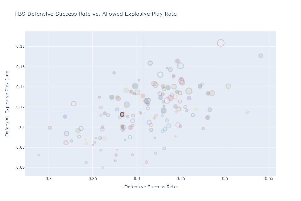
The FBS average success rate is 41.0%, while Virginia Tech allows success on 38.3% of plays.
Similarly, an explosive play is a pass that goes for 20 or more yards, or a run that goes for 10 or more yards.
The FBS average explosive rate is 11.6%, while Virginia Tech allows explosive plays on 11.2% of plays. Virginia Tech’s problem is not in explosive plays,
but mega-explosive, absolutely-backbreaking plays of 50 or more yards. Virginia Tech is tied for second in the most plays over 50 or more yards with 7 such plays (alongside Marshall, South Florida, Arkansas State, and Central Michigan), trailing only UMass at 9. Weirdly enough, if you look at just plays of 30 or more yards, Virginia Tech is much closer to the average allowing only 11 total (tied for 67th overall with schools that range from Charlotte and App State, to Texas, Florida, and Kansas).
More concerning is that this damage is being down almost exclusively on the ground, where 5 of the 7 50+ yarders have been rushing attempts. Virginia Tech’s rushing defense allows over 220 yards per game and over 5 yards per carry – among the worst in P5 football.
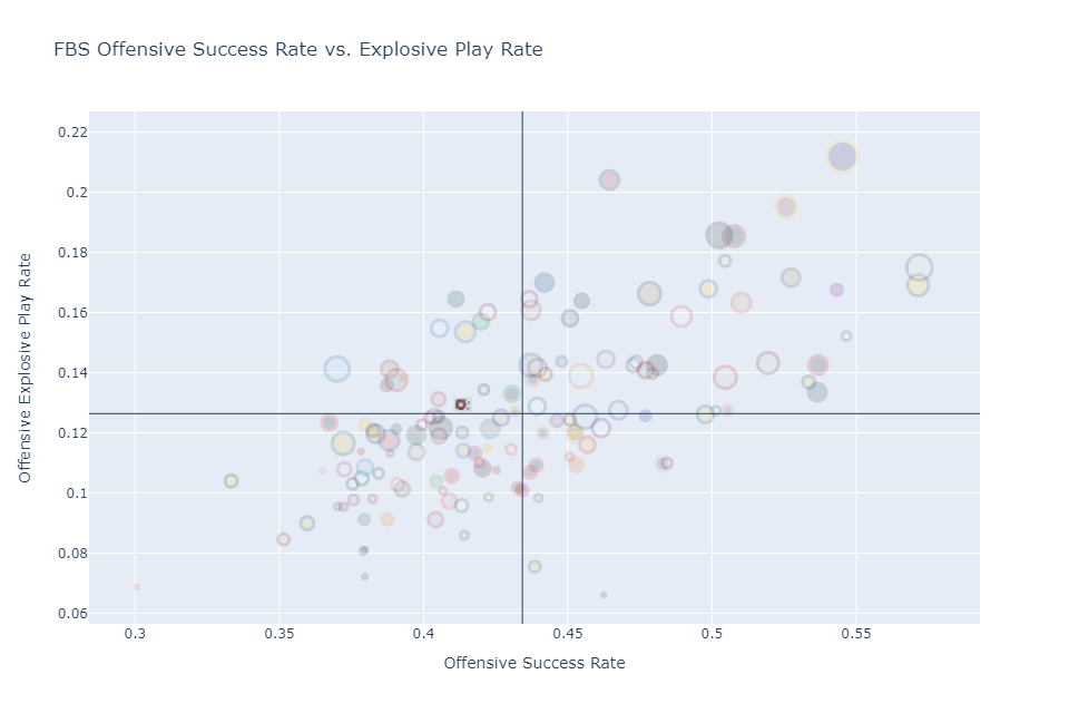
Virginia Tech’s offense struggled mightily under Offensive Coordinator Tyler Bowen and Quarterback Grant Wells in year one, leading the school to pick up big time transfers at QB (4* HS Kyron Drones, Baylor), WR (4* transfer Ali Jennings, Old Dominion; 3* transfer Jaylin Lane, Middle Tennessee; 3* transfer Da’Quan Felton, Norfolk State) and RB (3* transfer Bhayshul Tuten, NC A&T). While this leaned heavily on passing options, it betrayed many of Coach Pry’s insistence on becoming a much stronger rushing team after being too “easy to get a bead on” last season and lacking “creativity.” With Grant Wells going down before the half in Week 2, Virginia Tech’s grab bag offense faltered once again.
The new passing game was out the window with a QB who failed to break a completion percentage over 50% in high school in Kyron Drones, and the running game needed considerable work after nearly with negative rushing yards against Purdue. As a result, on the season Virginia Tech ranks 98th in success rate (39.8 % relative to the FBS average of 43.4%), and 88th in explosive rate (11.6% relative to the FBS average of 12.6%).

However, in week 4 against Marshall, the Virginia Tech offense started to show signs of life in the rushing game – averaging 6.1 yards per carry (184 yards on 30 attempts). Since becoming a more run-oriented offense Virginia Tech has improved their success rate to 42.0% (still below average) and their explosive rate to 12.9% (slightly above average).
Despite improvements on offense, and a defense that can be average on a down-to-down basis, Virginia Tech is rarely winning on both sides of the ball at the same time. Only one game this season (the 38-21 win over Pittsburgh) has Virginia Team won in EPA (expected points added) per play. A frequent critique of the Brent Pry era is that the team only plays one good quarter of football per game – something that Pry has often talked about in his press conferences regarding “complimentary football.” That still remains to be a major issue for this team.
Virginia Tech is averaging .111 EPA per play on offense and .201 EPA per play allowed on defense. If you compare EPA per play in each quarter, you find that Virginia Tech rarely wins both at the same or wins more than one quarter of a game. In this case we only win on average one quarter of a game (6 out of 24 total quarters). More worryingly, we only have one game this season where the offense has performed better than average for 3 quarters (Pitt) and one game where the defense has played better than average for 3 quarters (Marshall).
.png)
This matters because Virginia Tech still has a chance to finish strong. According to most metrics, the toughest part of Virginia Tech’s season is behind us. According to ESPN’s football playoff index, Virginia Tech (72nd in FPI/76th in SP+) has had the 35th hardest strength of schedule – but only the 72nd most difficult remaining schedule with games against:
Because of this, Virginia Tech still has a chance at respectability (if not outright bowl eligibility) if they are able to continuing improving on offense, and can turn some of the 50 yard plays into merely 30 yard plays. But it is going to take considerable effort from the players, and a level of coaching that we haven't seen yet from this staff.
Last week I took a lot at the “innovation capacity” of counties in Virginia by examining their share of knowledge-work and manufacturing jobs,
the percentage of residents over the age of 25 with a bachelor’s degree or higher, and the number of patents issued per capita (from 2000 to 2015).
What I found was that there was (unsurprisingly) a moderately strong correlation between a county’s innovation capacity score and
its relative proximity to a major research university (an R1 or R2 research university on the Carnegie Classification scale).
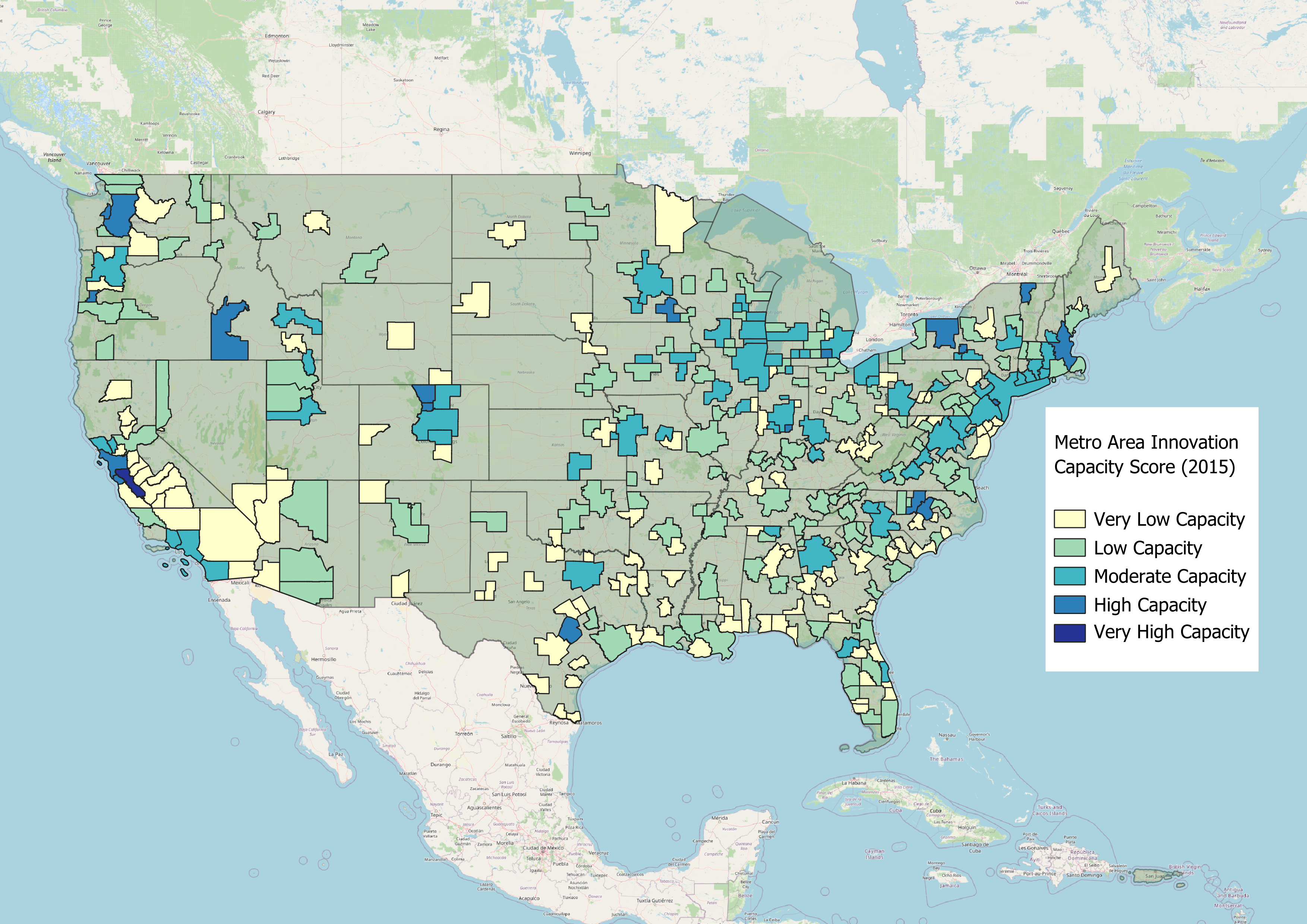
Today, I expanded that methodology to look at not just Virginia counties, but to all metropolitan statistical areas (MSAs) in the United States –
with some minor adjustments to the methodology. The results still resemble what you might expect; Silicon Valley dominates the top of the list
(with San Jose-Sunnyvale-Santa Clara #1 overall and San Francisco-Oakland-Berkeley #5), with other strong showings in research dominate metros
(Boston #9, Durham-Chapel Hill #10, Raleigh-Cary #12, Seattle #13).
There are three main factors that determine an MSAs overall success in these metrics:
One of the major changes between this and the original analysis was in calculating the innovative jobs score for each MSA. While I still used the same NAICS codes to categorize employment, I took the average of each sector over the years of 2014-2016. This change was made because of the high number of (D) depressed employment figures in the 2015 MSA dataset. Even with this change, about 30% of metro areas had at least one NAICS code that was a depressed value. While this was usually in smaller MSAs, it did impact some larger ones including Salt Lake City, San Jose, and Washington DC.
My solution was to impute a value based on the min, max, and mean values in each NAICS category. However, if this were a professional project and not for a blog, I would also to try reaggregate some of those values using more specific NAICS data from the Bureau of Labor Statistics Quarterly Census of Employment and Wages instead of relying solely on the Bureau of Economic Analysis’s Personal Income and Employment by County and Metropolitan Area dataset. I only included metro areas that were missing 2 or fewer NAICS employment categories, even after imputing data.
Another issue I ran into was the changing nature of MSA codes and definitions. To calculate the patents issued per capita and the educational attainment rate, I used American Community Survey data. I used 5-year estimates from 2015, as this was the last year of patent data available at the MSA level. However, there were some metro areas that changed from 2015 to 2023, which caused me to drop some areas from the overall analysis. An example of this is the Poughkeepsie-Newburgh-Middletown, NY MSA which was an MSA except for the years of 2013-2018, when it was considered part of the New York City-Newark-Jersey City, NY-NJ MSA.
Additionally, I restricted the final output to only including metro areas with a population of 300,000 or more. While this removes some of the smaller/rural/university focused MSAs, it provides a more accurate look at the regional economic drivers. It is worth noting that on a per capita basis, without restricting for population, Corvallis, OR and Burlington, VT are two of the top five innovation capacity metro areas.
Viewing the map as a whole you start to see alignment with what we know about existing regional economies: moderate to strong capacity for jobs and innovation in the ACELA corridor from Washington DC to Boston, moderate capacity throughout the industrial Midwest, deep challenges in the south (with the exceptions of the Research Triangle and Charlotte in North Carolina; Atlanta, GA; and Austin, TX, and existing tech hubs in the Pacific Northwest and Silicon Valley. The big difference is the sources of high innovation capacity and competitiveness from smaller MSAs and other MSAs not traditionally thought of as “innovative” at the national level: Boulder, CO; Boise, ID; and Manchester-Nashua, NH to name a few.
This matters because a simple regression on the median household income of an MSA in 2015, relative to its population and each component of the innovation capacity score shows that larger MSAs with higher innovation capacities have a statistically significant higher median household income.
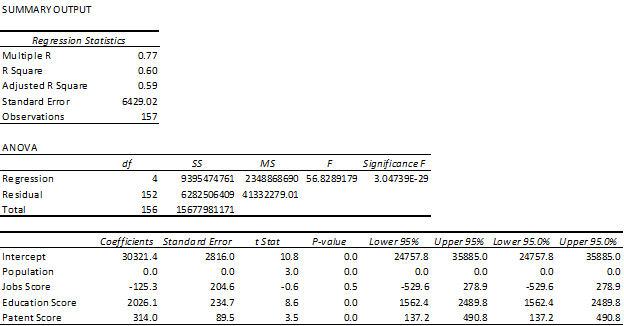
Only the jobs score was not a statistically significant predictor of median household income, which is not necessarily surprising given that that data had significant challenges in its reliability. While this isn’t the most robust analysis, nor something I would be submitting to the NBER – I do think it makes a strong case to as to the importance of investing in higher education, specifically regarding research and development, as well as high impact employment sectors. However, just because there is evidence that these factors positively impact economic development does not mean that every MSA is situated to become the next Silicon Valley. To do so would ignore the many historical reasons (natural resources, infrastructure, etc.) that these institutions and industries settled into their respective geographies in the first place.
For today's data blog, I wanted to try to focus on an interesting dataset I found from the U.S. Patent Office's Patent Technology Monitoring Team (PTMT).
The PTMT periodically releases data on patent activity throughout the country.
This includes a breakdown of utility patents issued by counties, metro areas, and states.
Although the smaller geographies haven't been updated since 2015,
I still wanted to see if I could use this data to better understand the regional implication of patents and innovation.
What I came up with was a simple metric called the innovation capacity score, which takes into account three variables:
- the total number of patents issued from 2000-2015 by county per capita;
- educational attainment of the county (2015)
- innovation jobs score (the mix of manufacturing, knowledge-work, and professional/scientific/technical service jobs as a share of the workforce, 2015).
I added the three components together, and mapped them along with the major colleges and universities in Virginia,
using the Carnegie Classifications of Institutions of Higher Learning (R1, R2, Special Purpose Research, and Doctoral/Professional Universities [formerly R3]).
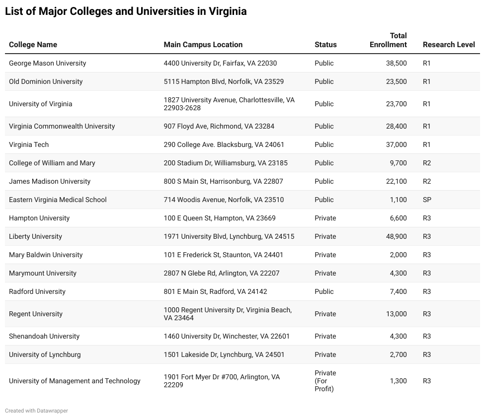
By doing so, we can start to quantify the advantage of having a major research institution has for a local economy.
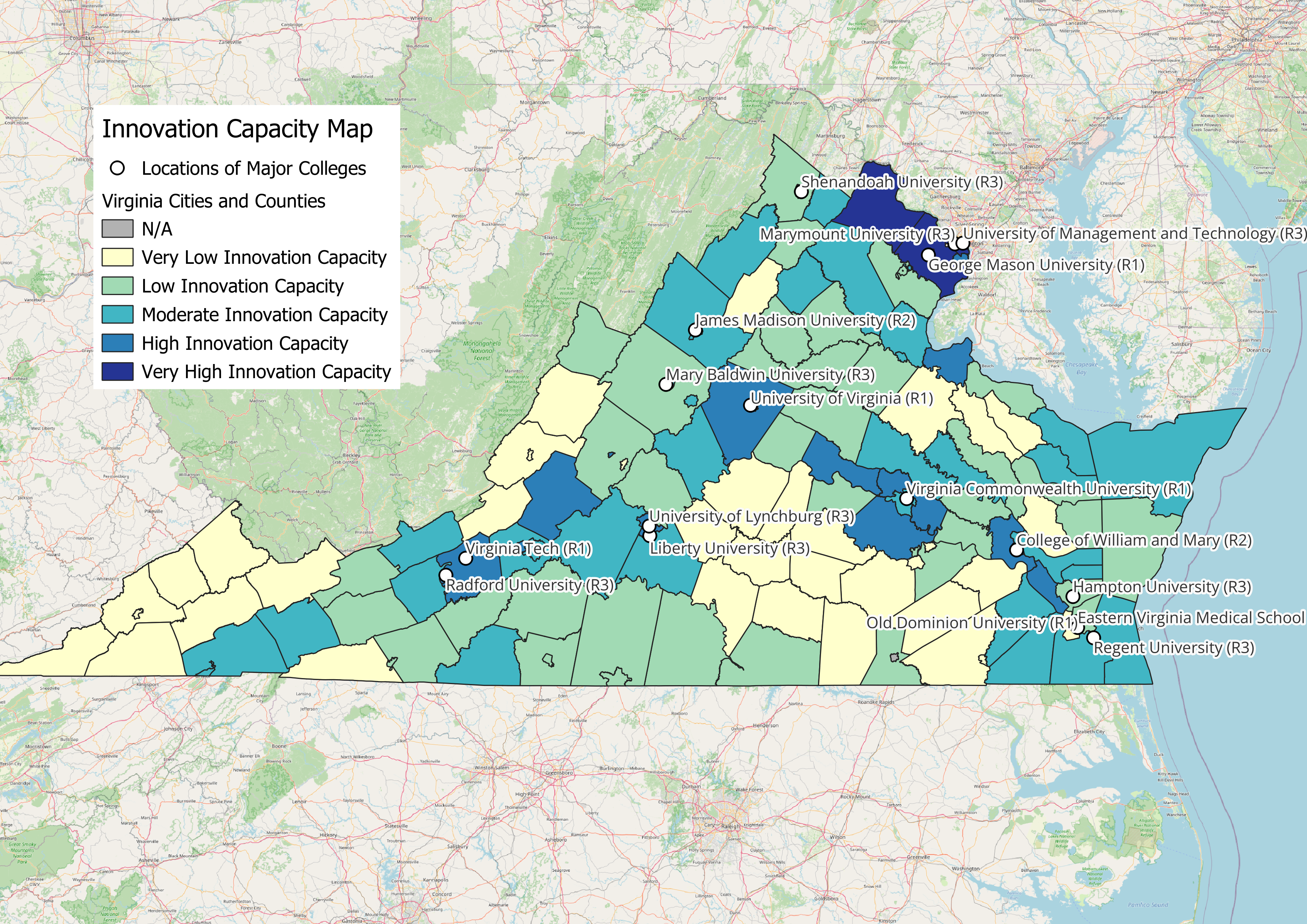
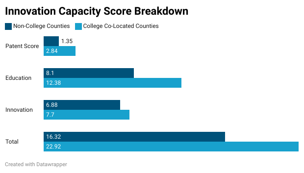
The average innovation capacity score was 19.32, which using the Jenks Natural Breaks score above, places it at the bottom end of the “Moderate Innovation Capacity” level. For counties that are within 25 miles of Virginia’s major universities, the average score was 22.92 which is over 6 points higher than the average for counties not near major universities, at 16.32. Counties near major universities scored higher on every component of the index, relative to the average and to non-college located counties.
One caveat worth mentioning is that the methodology for placing counties near major universities leaves is based on the centroid of the county, and not the location of the county seat or most populated areas. It is compared to the address of the university’s main campus (and does not consider alternative campus locations such as Virginia Tech and the University of Virginia’s northern Virginia locations).
Because of this decision, Loudoun County, the fourth most populated county at the time of the study (2015) and one of the richest counties in the United States is considered non-college located. However, if you take the county seat Leesburg as the point of comparison, Loudoun becomes a college-located county (nearest George Mason University). 70.8% of patents from 2000-2015 came from counties co-located near universities with the remaining 29.2% coming from the rest of the Commonwealth. If you include Loudoun as a co-locating county, only 10.0% of patents came from non-college located areas.
Similarly, you can breakdown the final Innovation Capacity Score by county size. I used the 75th percentile of population as the cutoff between large and small populace counties (above or below about 55,000 residents). While this closes the gap in terms of patents issued, it does not improve the gaps in educational attainment and innovative job availability. This makes some sense as there are colleges and universities located in small counties that produce patents (Virginia Tech in Montgomery County and the University of Virginia in Albemarle County to name a few). However, these areas are not necessarily keeping and retaining those graduates in the local job market – resulting in lower educational attainment and lower numbers of what we deemed innovative jobs.
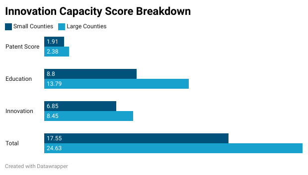
This is a massive challenge in economic development, most easily summed up by the question: “Do people follow jobs, or do jobs follow people?" How do small counties, especially counties without major colleges and universities, grow and attract talent and companies? These are the kinds of decisions that aren’t easily solved, but hopefully we can use data to contemplate better solutions.
Home Mortgage Disclosure Act (HDMA) data shows that the median property values for homebuyers are increasing at a rate that is outpacing income growth in the Richmond MSA from 2018 to 2022. This only applies to originated loans (where the median income for homebuyers was nearly $17,000 higher than the $81,400 median household income for the Richmond MSA in 2022), so you can imagine the difficulty that first-time homebuyers and low- or moderate-income (LMI) homebuyers are facing in this market.
But there are things we can be doing now at the local level to help with this burden, including:
1) Down-payment and closing cost assistance programs, with a particular focus on first-time homebuyers and/or first generation homebuyers.
2) Encourage banks to use creative new mortgage products to assist LMI and households by using Special Purpose Credit Programs.
3) Expanding homeownership opportunities in conjunction with "development with displacement" practices.
4) public investment in affordable housing through bond financing.
Yesterday was the release of the American Community Survey 1-year estimates for 2022, which got me thinking it is time
I better understood my new place of residence: Richmond, VA. Although I ended up looking at the census tract,
5-year estimates from 2021, I decided to make a community needs index for Richmond based on a variety of factors
like the methodology used by the Allegheny County Department of Human Services Community Needs Index.
The variables I included were:
· Single mother led households,
· Educational attainment for people over the age of twenty-five,
· Homeownership rate,
· Tract median family income as a percent of area median income; and,
· Tract median home value as a percent of the area median home value.
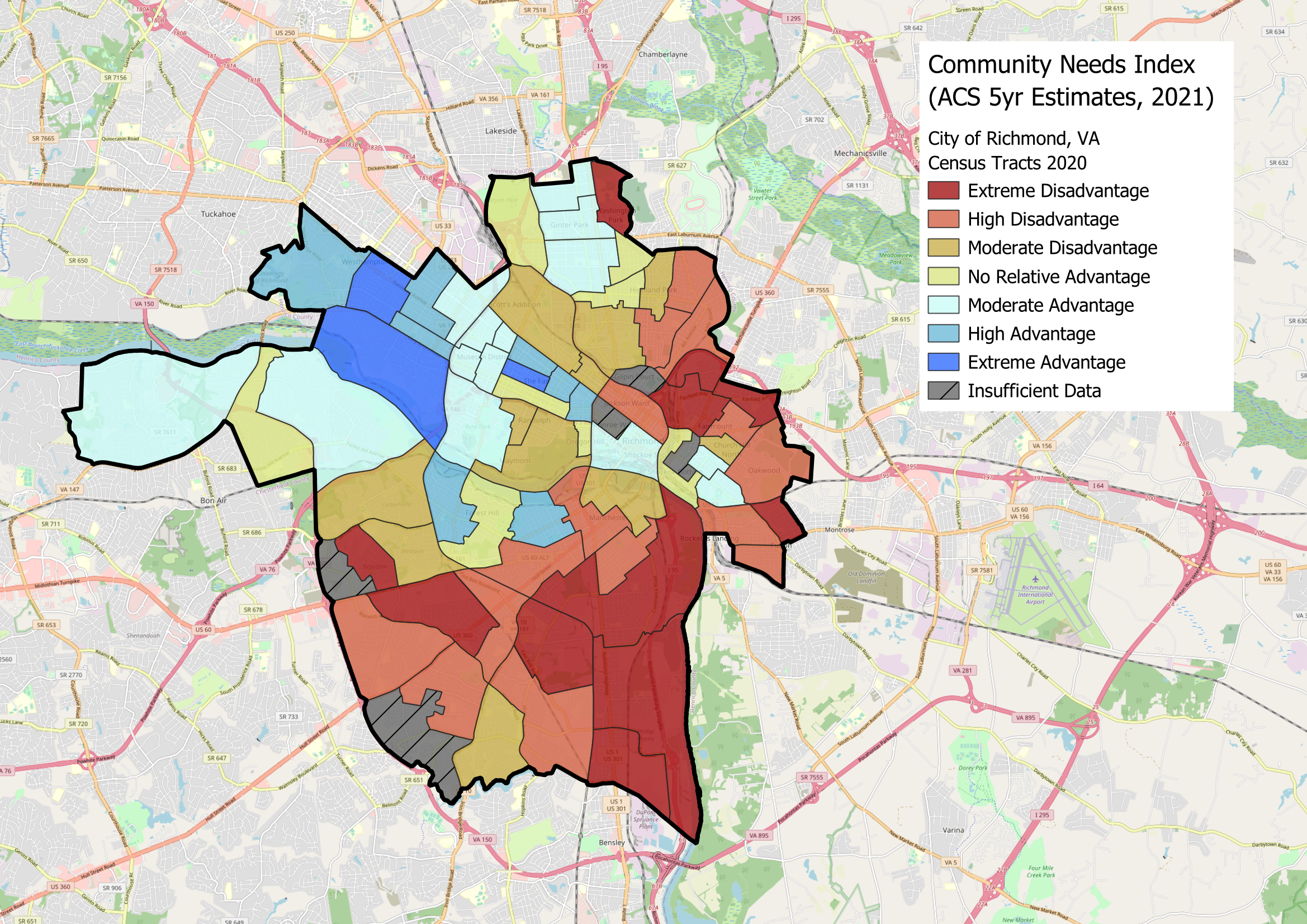
Unsurprisingly given the history of Richmond, the results speak for themselves. There is a strong correlation between being below average in the variables listed above compared to the tract’s population of Black residents in 2021. While this map focuses just on the City of Richmond, if you extend it to the Greater Richmond Area, the results stay about the same. My goal is to continue to build on this initial analysis by looking more into real estate transactions and mortgage data, but I wanted to start here – even if it isn’t anything groundbreaking.
Housing policy is the key to wealth building and remediating the racial and economic inequalities that continue to exist in Richmond. Whether its programs like the WORTH Initiative or looking at deferred home maintenance and repairs, there is so much that can be done here that can make a positive impact without contributing to the region’s massive history of gentrification and displacement.
Pre-pandemic Pittsburgh had one of the strongest bus transit systems in the county.
Unfortunately, its recovery has been just as slow as the other major transit agencies.
According to the National Transit Database's raw monthly ridership figures, the Pittsburgh Regional Transit system
(formerly the Port Authority of Allegheny County, as it is still referred to in the data)
had one of the strongest bus ridership figures per capita in the last full year of data from before the pandemic.
Specifically this was looking at transit agencies that: 1) operated in urbanized areas (UZAs) with a total population greater than 500,000; and 2)
completed at least 65,000,000 unlinked bus passenger trips from 2002 to June 2023.
Of the more than 800 unique transit authorities in the dataset, there were 112 active authorities that fit the above criteria. In 2019, PRT conducted approximately 56,350,000 bus trips, which equates to about 32.3 trips for every resident of the Pittsburgh metro area. That was the fifth highest per capita bus service of 2019, and coming from the smallest metro area in the top 10.
As you can see, even with a 42.5% reduction in bus passengers from pre-pandemic 2019 to 2022, Pittsburgh remains in the top 10 for passenger bus trips per capita. However, this may understate Pittsburgh's public transportation recovery due to the PRT's over-reliance on buses relative to light rail - where Pittsburgh trails heavily in per capita ridership and has had an even more anemic ridership recovery.
According to the 2019 American Community Survey Data, about 17% of the workers over the age of 16 within the City of Pittsburgh commuted to work by public transportation. But of those commuted to work on public transportation:
over half (53.1%) made less than $35,000 a year
less than a third owned homes (31.8%)
were predominantly women (57.3%)
and more likely to work in either the healthcare/education/social services industry (30.5%) or administrative or food services industry (17.3%).
This is critically important to remember when considering the demographics of who has left Pittsburgh in recent years. Recovering to those pre-pandemic levels will be harder as people are pushed further and further from the economic core of Pittsburgh. This will also be made tougher by the significant losses in buses operated by PRT - down almost 40% from 829 vehicles operated in maximum service 2002 to 498 in May 2023.
Part of Pittsburgh's existing success in public transportation stems from the fact that it is not solely used by daily workforce commuters. Ridership includes students who attend many of the schools within Pittsburgh, as well as the (albeit-limited) light rail service that primarily connects Downtown Pittsburgh with the stadiums on the North Shore and the residential areas of the South Hills. Having discretionary commuters is a worthy goal of every transportation agency, and one that has shown to reduce the stigmatization of public transportation in the United States.
Some cities used grant and pandemic recovery money to test free bus fares with relative success. Notable in the table above: Tucson, AZ has nearly recovered to their pre-pandemic ridership levels while maintaining free fares throughout at least 2023. Smaller city transit agencies like in Richmond, VA and Raleigh, NC have experienced relatively quicker recoveries (although still not to pre-pandemic levels) through free fare systems, while larger transit agencies such as the Denver Regional Transportation District in Denver, CO, the Massachusetts Bay Transportation Authority in Boston, MA, and the Metropolitan Transportation Authority in New York are experimenting with free fare pilot programs to various extents this summer.
Additionally, work like removing parking minimums and giving preference to transit oriented development can be key to enhancing existing transit systems - and is in line with the work advocated for by organizations like Pittsburghers for Public Transit, BikePGH, and Pittsburgh Community Reinvestment Group - signatories to Pittsburghers for Public Transit's 100 Days Transit Platform.
While much of this article paints a relatively rosy picture of pre-pandemic public transportation in Pittsburgh, it does not mean that the system was perfect or infallible. Bus bunching is still a major issue, as are equity concerns in the Bus Rapid Transit project for Downtown-Uptown-Oakland such as the removal in the Edgewood/Swissvale area that would no longer be serviced by the P3, or the underutilized light-rail system that operates at less capacity and at higher cost than other light-rail services, and so many other valid and legitimate concerns.
We need to continue to speak up for what is right, continue to push local elected officials on their promises and hold them accountable for their failures, especially with regards to public transportation and housing. But we also need to recognize the strengths that exist within the system, and use a data-informed approach that centers on real human experiences to do so. Hopefully, this article can be a good starting point for some of those discussions as Pittsburgh and Allegheny County head into election season this fall.
See original article here for in text citations.
Here is an aggregated look at the number of total workers residing in a neighborhood or municipality in Allegheny County by monthly earnings.
It uses the Longitudinal Employer-Household Dynamics (LEHD) Origin-Destination Employment Statistics data (residence area characteristics only)
from 2010-2020, aggregated from census block groups to combined neighborhoods and municipality level through census tracts.
It should serve
as a good companion to the affordability map I posted earlier this week.

Some interesting places to take a look at include Upper, Central, and Lower Lawrenceville, Bloomfield, and the Strip District in the City and Dormont and Wilkinsburg in the County.
Even though I don't live in Pittsburgh anymore, the Irish Centre development has reminded me that we don't do a great job of discussing what affordability
means at a neighborhood/community level and why that matters when housing projects are announced.
So I created this map that looks at the median home value relative to the MSA median household income for census tracts in Allegheny County,
according to the 2021 American Community Survey data
(5-year estimates).
At the MSA level, the price-to-income ratio for the median home price to the median income is 2.54,
but that isn't true in each census tract. The places that are most affordable are the areas of Allegheny County that are historically
redlined and marginalized communities, facing the most disinvestment -
which I would add in my opinion is not an accident.
Unsurprisingly, these are also the communities that typically saw a lot of population decline from 2010-2020.
(For more information, check out Chris Briem's 2020 Census Redistricting Data Extracts on the Western PA Regional Data Center's website.)
The most unaffordable places are the suburbs to the north and west of Pittsburgh,
as well as the areas in the East End around Pitt and CMU.
Those neighborhoods/communities in-between are becoming less and less frequent, as neighborhoods like Brookline, Bloomfield, Greenfield, and Garfield are seeing home values go up. The same is true in the county, particularly in the boroughs and townships in the South Hills.
Just wanted to give a little context towards the quotes that were attributed to Pittsburgh Community Reinvestment Group in this piece [titled "Study: Black homeownership rate in Pittsburgh remains disproportionately small"]. Penn Hills, Monroeville, Stowe, McKeesport, McKees Rocks, and Turtle Creek all experienced a net increase in Black population, while East Liberty, Lincoln-Lemington, and Garfield lost Black population from the 2010 Census to the 2020 Census.
However, these moves (either in or out) are not all equal. At the time I spoke with the author of this article, the latest ACS data was from 2020. I had noted that Penn Hills, Monroeville, and Stowe had seen net increases in Black population AND significant gains in median household income for Black households over the previous 5-year ACS period (Table B19013B on the census data site for those wondering).
So much so that the median household income for a Black household in Penn Hills ($52,353), Monroeville ($64,365), or Stowe ($48,642) are nearly twice that of the City of Pittsburgh ($27,365). At the same time, areas like McKeesport ($26,108), McKees Rocks ($24,531), and Turtle Creek ($22,423) saw increases in Black population, but are areas that still below median household income for Black households in Pittsburgh. This is an important distinction.
Similarly, I would categorize the neighborhoods that experienced significant Black population loss differently. Areas like East Liberty and Upper Lawrenceville, that lost 34.3% and 79.5% of their Black populations respectively, saw clear evidence of gentrification and displacement. Garfield also saw evidence of gentrification and displacement, but not necessarily to the degree or with the amount of media coverage as East Liberty.
However, areas like Lincoln-Lemington and Homewood North also experienced significant Black population declines without the noticeable material gains experienced in East Liberty, Lawrenceville, and Garfield.
The reason I bring this up is because terms like gentrification and displacement get used a lot in the space, and it can present issues with how we discuss real challenges faced by real families and individuals. I regret that I may not have expressing my ideas correctly when I talked to Tim Grant a couple of months ago. But this is important because a lot of attention is given to communities going through gentrification, while much less attention is given to areas seeing displacement without material change. We should not conflate the two. To do so may ignore the realities of disinvested communities and neighborhoods that are prone to high concentrations of poverty, community violence, and continued racial segregation. These issues affect the movements of populations in the region just as much as housing affordability. No one should have to choose between a safe neighborhood and an affordable neighborhood.